12. What is the Bellman-Ford algorithm for finding single source shortest paths? What are its main advantages over Dijkstra? Use C . Algorithm, Question, Explanation, Solution. At toptal-com .
By: Chrysanthus Date Published: 3 Feb 2026
A negative cycle is a path that can be followed in cycles, where the sum of the edge weights is negative. Using the basic Bellman-Ford algorithm on a graph with negative cycles will not produce a result of shortest paths because in a negative cycle, one can always go one more cycle and get a shorter path. Luckily, the basic Bellman-Ford algorithm can be modified to safely detect and report the presence of negative cycles; but that will not be addressed in this article
An edge weight is the value of the edge.
This is a teaching document, so for an actual interview, summarize all what is given in this document.
Explanation of the Basic Bellman-Ford Algorithm
In this section, Bellman-Ford Algorithm is illustrated first, before the algorithm is given as a series of steps. After that, the code is given based on the illustration (manual-run-through).
Manual-Run-Through of Bellman-Ford Algorithm
Consider the following network graph:
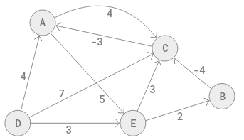
There
are 5 vertices and there are 9 edges. The value of each edge is
indicated by the edge. A directed graph is a graph where each edge has a
direction, which is indicated by an arrow-head. Movement cannot take
place in the reverse direction. The weight of an edge may be positive or
negative. Whether it is negative or not, the arrow-head is for the
forward direction of movement.
V is the number of vertices and E is the number of edges. Do not confuse between edge and edge-weight.
For this problem, the source is D, and the shortest distance from D to each of the other vertices has to be determined, bearing in mind that some edges have negative values in their forward directions.
The first thing to do is to set the distance from D to D itself, as 0; then set the distance to each of the other vertices from D, as positive infinity, as it assumes the algorithm is not yet aware of their presence. Infinity is an unimaginably large number. The following image shows this:
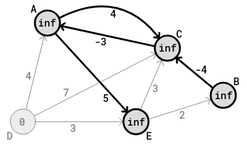
So,
the distance from D to D is 0. The cost of vertex D is said to be 0.
The distance from D to E is infinity; the distance from D to A is
infinity; the distance from D to C is infinity; the distance from D to B
is infinity (and so on). These distances are written in their
corresponding vertex circles. An assumed sum distance written in the
circle of a vertex is known as the cost of that vertex. So the distance
(summed) or cost of each of the vertices from D, at the start of the
algorithm is infinity.
The table corresponding to this initial state is:
The table corresponding to this initial state is:
| Previous Vertex | Vertex | Cost |
|---|---|---|
| A | infinity | |
| B | infinity | |
| C | infinity | |
| D | 0 | |
| E | infinity |
At the beginning, list all the vertices in the middle column in ascending order.
Rounds
Bellman-Ford Algorithm is done in rounds. When there are V vertices, the number of rounds is V - 1. There are 5 vertices here, and so the number of rounds is 4 = 5 - 1.
In each round, all the edges have to be checked, one time. The different edges from the diagram are:
(D-A), (D-C), (D-E), (A-E), (A-C), (E-B), (E-C), (B-C), (C-A);
all 9 edges. The order in which the edges are arranged from left to right, in this line, does not matter. Note that the first letter is the start of a particular edge and the last (second) letter is the end of that same edge, in the forward direction of the arrow-head; though some edge weights might have negative values. In the table, the particular edge start letter is in the first column, while the end (second) letter is in the second (middle) column, row by row. So, for a particular edge, the left (first) letter is the previous vertex and the right (end) letter is the vertex in question. The cost of the end (second or right) vertex is in the third column in the same row. As the algorithm proceeds in a round, the start or previous letter in a row, in the first column may change, indicating a neighboring edge to the same end vertex (letter).
In any round, all the vertices (9) are assessed to know the assumed cost for each vertex. The cost of each vertex is the assumed distance from the source, D. Always bear in mind that it is the minimum distance from D that is looked for. And so, when a new cost is found to be lower than a former cost, the new cost replaces the former cost for that vertex. That is called relaxation.
At the beginning of the algorithm, the cost of D is 0 and the cost of the other vertices are each infinity.
Round 1
The list of edges is:
(D-A), (D-C), (D-E), (A-E), (A-C), (E-B), (E-C), (B-C), (C-A)
copied from above.
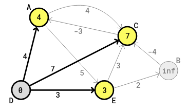
With the edge (D-A), the cost of A should become 4 = 0+4 and 4 is less than infinity. So 4 has to replace infinity in the circle of A in the diagram. In the A (middle column) row in the table, the value in the third column has to become 4 and the value in the first column has to be D, the previous (or start) letter of the current edge.
With the edge (D-C), the cost of C should become 7 = 0+7 and 7 is less than infinity. So 7 has to replace infinity in the circle of C in the diagram. In the C (middle column) row in the table, the value in the third column has to become 7 and the value in the first column has to become D, the previous (or start) letter of the current edge.
The reader should be filling the values in the table in his/her rough work, as the round continues.
With
the edge (D-E), the cost of E should become 3 = 0+3 and 3 is less than
infinity. So 3 has to replace infinity in the circle of E in the
diagram. In the E (middle column) row in the table, the value in the
third column has to become 3 and the value in the first column has to
become D, the previous (or start) letter of the current edge. The
following diagram shows the current state:
With
the edge (A-E), the cost of E should become 9 = 4+5 (the 4 here is the
current cost of A in the circle of A). 9 is not less than 3, the assumed
shortest cost of E. So 9 does not replace 3 in the circle of E in the
diagram. In the E (middle column) row in the table, the value in the
third column remains at 3 and the value in the first column remains at
D, the previous (or start) letter of a neighboring edge.
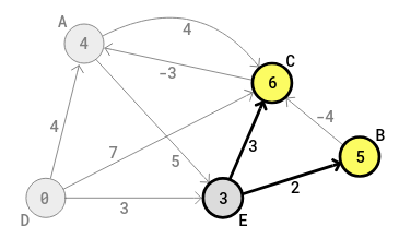
With the edge (E-B), the cost of B should become 5 = 3+2 (the 3 here is the current cost of E in the circle of E) and 5 is less than infinity, the assumed shortest cost of B. So 5 replaces infinity in the circle of B in the diagram. In the B (middle column) row in the table, the value in the third column becomes 5 and the value in the first column becomes E, the previous (or start) letter of the current edge. At this point, still in the first round, there is no longer any infinity value in the third column of the table.
With the edge (E-C), the cost of C
should become 6 = 3+3 (the first 3 here is the current cost of E in the
circle of E) and 6 is less than 7, the assumed shortest cost of C. So 6
replaces 7 in the circle of C in the diagram (relaxation). In the C
(middle column) row in the table, the value in the third column becomes 6
(from 7) and the value in the first column becomes E (from D), the
previous (or start) letter of the current edge (is E). The following
diagram shows the current state, in still the first round:
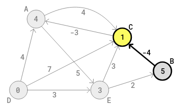
With
the edge (B-C), the cost of C should become 1 = 5+-4 = 5-4 (the 5 here
is the current cost of B in the circle of B) and 1 is less than 6, the
assumed shortest cost of C. So 1 replaces 6 in the circle of C in the
diagram. In the C (middle column) row in the table, the value in the
third column becomes 1 (from 6) and the value in the first column
becomes B (from E), the previous (or start) letter of the current edge
(is B). The following diagram shows the current state in still the first
round:
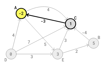
With
the edge (C-A), the cost of A should become -2 = 1+-3 = 1-3 (the 1 here
is the current cost of C in the circle of C) and -2 is less than 4, the
assumed shortest cost of A. So -2 replaces 4 in the circle of A in the
diagram. In the A (middle column) row in the table, the value in the
third column becomes -2 (from 4) and the value in the first column
becomes C (from D), the previous (or start) letter of the current edge
(is C). The following diagram shows the current and final state in the
first round:
The Bellman-Ford algorithm now has checked each edge 1 time. Round one ends ! The final state of the table in round 1 is:
| Previous Vertex | Vertex | Cost |
|---|---|---|
| C | A | -2 |
| E | B | 5 |
| B | C | 1 |
| D | 0 | |
| D | E | 3 |
Note that there is no letter in the first column cell of row D, as the distance from D to D is 0. The cost of D is 0.
Round 2
There has to be 4 rounds for 5-1 = 4 of V-1. In each round, all the edges have to be checked again for shortest path from D. Each edge is checked or assessed once. The edges are:
(D-A), (D-C), (D-E), (A-E), (A-C), (E-B), (E-C), (B-C), (C-A);
copied from above.
With the edge (D-A), the cost of A should become 4 = 0+4, but 4 is not less than -2. So 4 does not replace -2 in the circle of A in the diagram. In the A (middle column) row in the table, the value in the third column remains at -2 and the value in the first column remains at C, the previous (or start) letter of a neighboring edge.
With the edge (D-C), the cost of C should become 7 = 0+7, but 7 is not less than 1. So 7 does not replace 1 in the circle of C in the diagram. In the C (middle column) row in the table, the value in the third column remains at 1 and the value in the first column remains at B, the previous (or start) letter of a neighboring edge.
The final table for round 1 has not yet changed.
With the edge (D-E), the cost of E should become 3 = 0+3, but 3 is not less than the 3 which is still at E. So 3 does not replace the 3 which is still in the circle of E in the diagram. In the E (middle column) row in the table, the value in the third column remains at 3 and the value in the first column remains at D, the previous (or start) letter of the current or neighboring edge. Note that the table at its last state in round 1 has still not changed and the state of the final diagram in round 1 has still not changed. The current diagram in this second round is still what the algorithm had at the end of round 1. It is still:
With the edge (A-E), the cost of E at this point in this second round, should become 3 = -2+5 (the -2 here is the current cost of A in the circle of A). This new 3 is not less than the old 3, which is the assumed shortest cost of E, from the first round. So the new 3 does not replace the old 3 in the circle of E in the diagram. In the E (middle column) row in the table, the value in the third column remains at 3 and the value in the first column remains at D, the previous (or start) letter of a neighboring edge.
With the edge (A-C), the cost of C at this point in the second round, should become 2 = -2+4 (the -2 here is the current cost of A in the circle of A). 2 is not less than 1, the assumed shortest cost of C, from the first round. So 2 does not replace 1 in the circle of C in the diagram. In the C (middle column) row in the table, the value in the third column remains at the last value of 1 from the first round, and the value in the first column remains at the last value of B, the previous (or start) letter of a neighboring edge, from the first round.
With the edge (E-B), the cost of B should become 5 = 3+2 (the 3 here is the current cost of E in the circle of E). The 5 here is the same 5 in the first round, the assumed shortest cost of B. This same 5 is not less than itself. So it does not replace itself in the circle of B in the diagram. Do not forget that the idea is to look for the shortest path within a round and in the next round. In the B (middle column) row in the table, the value in the third column remains at 5 and the value in the first column remains at E, the previous (or start) letter of the current edge.
With the edge (E-C), the cost of C should become 6 = 3+3 (the first 3 here is the current cost of E in the circle of E), but 6 is not less than 1, the assumed shortest cost of C, at this point. So 6 does not replace 1 in the circle of C in the diagram - in this second round. In the C (middle column) row in the table, the value in the third column remains at 1 and the value in the first column remains at B, the previous (or start) letter of a neighboring edge (is B). The following diagram shows the current state (no change), in still the second round:
With the edge (B-C), the cost of C should become 1 = 5+-4 = 5-4 (the
5 here is the current cost of B in the circle of B) and the new 1 is
not less than the old 1 already in C, the assumed shortest cost of C.
So 1 does not replace 1 in the circle of C in the diagram. In the C
(middle column) row in the table, the value in the third column
remains at 1 and the value in the first column remains at B, the
previous (or start) letter of the current edge (is B). The following
diagram shows the current state (no change) in still the second
round:
With the edge (C-A), the cost of A should become -2 = 1+-3 = 1-3 (the
1 here is the current cost of C in the circle of C) and the new -2 is
not less than the old -2, the assumed shortest cost of A. So the new
-2 does not replace the old -2 in the circle of A in the diagram. In
the A (middle column) row in the table, the value in the third column
remains at -2 and the value in the first column remains at C, the
previous (or start) letter of the current edge (is C). The following
diagram shows the current and final state in the second round:
The Bellman-Ford algorithm now has checked each edge 1 time. Round two ends! The final state of the table in round 2 is:
| Previous Vertex | Vertex | Cost |
|---|---|---|
| C | A | -2 |
| E | B | 5 |
| B | C | 1 |
| D | 0 | |
| D | E | 3 |
Note that there is no letter in the first column cell of row D, as the distance from D to D is 0. The cost of D is 0.
It is important to note here, that though there were some changes in the calculations in the second round, the final result (of the diagram and table) has not changed from that of the first round.
Now, with other similar graph networks, up to 4 rounds, 5-1 (V-1) have to be done to have the final and stable state. However here, only two rounds had to be made to have the final and stable state.
With the Bellman-Ford algorithm, once the new round has no difference in final diagram and final table, with the final diagram and final table of the preceding round, then the algorithm should stop and not waste any more time checking more rounds and edges. It should stop because the diagram and table have become stable, and further rounds will not bring in any new change.
If the number of rounds go beyond V-1, then there is at least one negative cycle in the graph. However that is not addressed in this document.
So the final state of the Bellman-Ford algorithm for the above problem has been attained. The next issue is to obtain the shortest path from D, to reach each of the other vertices from the final state (the table). The shortest path should be obtained both in path-weight and order of vertices.
Obtaining the Shortest Path of the Other Vertices
The shortest path from D to D is 0, from definition.Shortest Path Weight of other Vertices
To obtain the shortest path weight of the other vertices, use the final state of the table at the last round (for the above problem, second round). Each value in the third column is the shortest path-weight from D, and not from the corresponding table row value in the first column.Locate the vertex (letter) in the middle column of the table. The value in the third column of the same row is its shortest path-weight from D. This can also be read from the circle of the vertex from the final diagram of the last round (for the above problem, second round).
The diagram can also be used instead of the table, if the costs of the different vertices were updated as the edges were assessed (checked).
The shortest path weight of A is -2 and not 4. This is a graph with directed edges, some of whose values are negative. The shortest path weight of C is 1 and not 7.
The shortest path weight of B is 5. That coincidentally can be seen from the given diagram. The shortest path weight of E is 3. That coincidentally can also be seen from the given diagram.
Shortest Path by Order of Vertices
It is not
straight forward to obtain the shortest path by order of vertices, from
the final diagram. So the final table (state) has to be used. The
shortest path by order of vertices to the other vertices is obtained
from the table, while visualizing the final diagram, though visualizing
the final diagram is not absolutely necessary here. The final diagram
and table are repeated from above; thus:
| Previous Vertex | Vertex | Cost |
|---|---|---|
| C | A | -2 |
| E | B | 5 |
| B | C | 1 |
| D | 0 | |
| D | E | 3 |
Obtaining
the shortest path order is done by backward movement in the table. To
obtain the shortest path order for any vertex other than the source
vertex, go to the middle column of the table and locate the vertex. In
the same row, go to the first column and identify the previous edge
vertex. From there, go to the middle column and locate that previous
vertex from the first column, in a new row. From that location in the
middle column and in the same row, identify the new previous edge vertex
in the first column. Keep repeating that movement until D is reached in
the first column. Present the vertices in forward order, from the
table, and without repeating a vertex.
For the shortest path of B , locate B in the middle column, second row in the table. The previous vertex that connects to B for the single corresponding edge for B, going backwards ultimately to D, is E, in the first column in the same (second) row. The weight of this edge is 2 (from the given diagram).
This previous vertex E, has to be located as the end vertex of an edge in the middle column. It is located in the middle column in row 5. The previous vertex for the single edge of interest that ends at E is D, in the same row (row 5). The weight of this edge is 3 (from the given diagram). D has been arrived at. Writing the path in forward order of vertices from the table (without repeating a vertex), gives:
D-E-B
Adding the path weights in forward order is:
3+2 = 5 (for D-E and E-B)
For the shortest path of A, locate A in the middle column, first row in the table. The previous vertex that connects to A for the single corresponding edge from A, going backwards ultimately to D, is C (not D), in the first column in the same (first) row. The weight of this edge is -3 (from the given diagram).
This previous vertex C, has to be located as the end vertex of an edge in the middle column. It is located in the middle column in row 3. The previous vertex for the single edge of interest that ends at C is B, in the same row (row 3). The weight of this edge is -4.
This previous vertex B, has to be located as the end vertex of an edge in the middle column. It is located in the middle column in row 2. The previous vertex that connects to B for the single corresponding edge for B, going backwards ultimately to D, is E, in the first column in the same (second) row. The weight of this edge is 2 (from the given diagram).
This previous vertex E, has to be located as the end vertex of an edge in the middle column. It is located in the middle column in row 5. The previous vertex for the single edge of interest that ends at E is D, in the same row (row 5). The weight of this edge is 3. D has been arrived at, in the first column. Writing the path in forward order of vertices from the table (without repeating a vertex), gives:
D-E-B-C-A
Adding the path weights in forward order is:
3+2+-4+-3 = 3+2-4-3= -2 (for D-E, E-B, B-C and C-A)
The path order and sum path weight of the remaining two vertices are determined in the same way.
- The cost from the source vertex to each of the other vertices is infinity, at the start of the algorithm.
- Produce a table with 3 columns, where the first column is for the previous vertex of an edge of interest, the middle column is for the end vertex for the same edge of interest, and the third and last column is for the temporary cost of the end vertex from D, temporarily ending with the edge of interest.
- Each edge in the whole graph has to be assessed in rounds.
- The maximum number of rounds is V-1 where V is the number of vertices.
- When each vertex is assessed in a round, the corresponding row cell in the third column of the table is updated appropriately with the cost.
- Once the new round has no difference in final diagram and final table, with the final diagram and final table of the preceding round, then the algorithm should stop, and not waste any more time checking more rounds and edges.
- If the number of rounds go beyond V-1, then there is at least one negative cycle in the graph.
For the shortest path of B , locate B in the middle column, second row in the table. The previous vertex that connects to B for the single corresponding edge for B, going backwards ultimately to D, is E, in the first column in the same (second) row. The weight of this edge is 2 (from the given diagram).
This previous vertex E, has to be located as the end vertex of an edge in the middle column. It is located in the middle column in row 5. The previous vertex for the single edge of interest that ends at E is D, in the same row (row 5). The weight of this edge is 3 (from the given diagram). D has been arrived at. Writing the path in forward order of vertices from the table (without repeating a vertex), gives:
D-E-B
Adding the path weights in forward order is:
3+2 = 5 (for D-E and E-B)
For the shortest path of A, locate A in the middle column, first row in the table. The previous vertex that connects to A for the single corresponding edge from A, going backwards ultimately to D, is C (not D), in the first column in the same (first) row. The weight of this edge is -3 (from the given diagram).
This previous vertex C, has to be located as the end vertex of an edge in the middle column. It is located in the middle column in row 3. The previous vertex for the single edge of interest that ends at C is B, in the same row (row 3). The weight of this edge is -4.
This previous vertex B, has to be located as the end vertex of an edge in the middle column. It is located in the middle column in row 2. The previous vertex that connects to B for the single corresponding edge for B, going backwards ultimately to D, is E, in the first column in the same (second) row. The weight of this edge is 2 (from the given diagram).
This previous vertex E, has to be located as the end vertex of an edge in the middle column. It is located in the middle column in row 5. The previous vertex for the single edge of interest that ends at E is D, in the same row (row 5). The weight of this edge is 3. D has been arrived at, in the first column. Writing the path in forward order of vertices from the table (without repeating a vertex), gives:
D-E-B-C-A
Adding the path weights in forward order is:
3+2+-4+-3 = 3+2-4-3= -2 (for D-E, E-B, B-C and C-A)
The path order and sum path weight of the remaining two vertices are determined in the same way.
Bellman-Ford Algorithm as a Series of Steps
- The cost from the source vertex to itself is 0.- The cost from the source vertex to each of the other vertices is infinity, at the start of the algorithm.
- Produce a table with 3 columns, where the first column is for the previous vertex of an edge of interest, the middle column is for the end vertex for the same edge of interest, and the third and last column is for the temporary cost of the end vertex from D, temporarily ending with the edge of interest.
- Each edge in the whole graph has to be assessed in rounds.
- The maximum number of rounds is V-1 where V is the number of vertices.
- When each vertex is assessed in a round, the corresponding row cell in the third column of the table is updated appropriately with the cost.
- Once the new round has no difference in final diagram and final table, with the final diagram and final table of the preceding round, then the algorithm should stop, and not waste any more time checking more rounds and edges.
- If the number of rounds go beyond V-1, then there is at least one negative cycle in the graph.
Basic Code for Bellman-Ford Algorithm
The Adjacency Matrix table for the above graph is:A B C D E
A 4 5
B -4
C -3
D 4 7 3
E 2 3
Excluding the include directives, there are six main code segments for the program. This does not include the main() function, where the given matrix is formed and the bellmanFord() function is called.
The Graph Class Code Segment
The first code segment produces a class for the graph.
The createGraph() Code Segment
This code segment (function) instantiates a graph object from the Graph class and returns the instance.
The addEdge() code segment
An edge here is the weight or distance from one vertex to a neighboring vertex. In the adjacency matrix, this is the value of the intersection cell of the row (index) of one of the vertices and the column (index) of the other vertex. This function (code segment) achieves that.
The addVertexData() Code Segment
This function (code segment) assigns to an index of interest, the corresponding letter (of the alphabet).
The bellmanFord() Code Segment
This function (code segment) is the core of the program. It performs the Bellman-Ford algorithm.
The freeGraph() Code Segment
This code segment (function) frees dynamic memory.
Complete Program for Basic Bellman-Ford Algorithm
The complete program is as follows:
#include <stdio.h>
#include <stdlib.h>
#include <string.h>
#include <limits.h>

#define MAX_VERTEX_DATA 10 // Maximum length of vertex data string

typedef struct {
    int size;
    int **adjMatrix;
    char **vertexData;
} Graph;

Graph* createGraph(int size) {
    Graph *g = (Graph*)malloc(sizeof(Graph));
    g->size = size;

    // Allocate memory for adjacency matrix
    g->adjMatrix = (int**)malloc(size * sizeof(int*));
    for (int i = 0; i < size; i++) {
        g->adjMatrix[i] = (int*)calloc(size, sizeof(int));
    }

    // Allocate memory for vertex data
    g->vertexData = (char**)malloc(size * sizeof(char*));
    for (int i = 0; i < size; i++) {
        g->vertexData[i] = (char*)calloc(MAX_VERTEX_DATA, sizeof(char));
    }

    return g;
}

void addEdge(Graph *g, int u, int v, int weight) {
    if (u >= 0 && u < g->size && v >= 0 && v < g->size) {
        g->adjMatrix[u][v] = weight;
        //g->adjMatrix[v][u] = weight; // For undirected graph
    }
}

void addVertexData(Graph *g, int vertex, const char *data) {
    if (vertex >= 0 && vertex < g->size) {
        strncpy(g->vertexData[vertex], data, MAX_VERTEX_DATA - 1);
    }
}

void bellmanFord(Graph *g, const char *startVertexData) {
    int startVertex = -1;
    for (int i = 0; i < g->size; i++) {
        if (strcmp(g->vertexData[i], startVertexData) == 0) {
            startVertex = i;
            break;
        }
    }

    if (startVertex == -1) {
        printf("Start vertex not found\n");
        return;
    }

    int distances[g->size];
    for (int i = 0; i < g->size; i++) {
        distances[i] = INT_MAX;
    }
    distances[startVertex] = 0;

    for (int i = 0; i < g->size - 1; i++) {
        for (int u = 0; u < g->size; u++) {
            for (int v = 0; v < g->size; v++) {
                if (g->adjMatrix[u][v] != 0 && distances[u] != INT_MAX &&
                    distances[u] + g->adjMatrix[u][v] < distances[v]) {
                    distances[v] = distances[u] + g->adjMatrix[u][v];
                    printf("Relaxing edge %s->%s, Updated distance to %s: %d\n",g->vertexData[u], g->vertexData[v], g->vertexData[v], distances[v]);
                }
            }
        }
    }

    // Print distances
    for (int i = 0; i < g->size; i++) {
        printf("Distance from %s to %s: %d\n", startVertexData, g->vertexData[i], distances[i]);
    }
}

void freeGraph(Graph *g) {
    if (g != NULL) {
        // Free each row of the adjacency matrix
        for (int i = 0; i < g->size; i++) {
            free(g->adjMatrix[i]);
        }
        // Free the adjacency matrix itself
        free(g->adjMatrix);

        // Free each vertex data string
        for (int i = 0; i < g->size; i++) {
            free(g->vertexData[i]);
        }
        // Free the vertex data array
        free(g->vertexData);

        // Finally, free the graph structure
        free(g);
    }
}

int main() {
    Graph *g = createGraph(5);

    addVertexData(g, 0, "A");
    addVertexData(g, 1, "B");
    addVertexData(g, 2, "C");
    addVertexData(g, 3, "D");
    addVertexData(g, 4, "E");

    addEdge(g, 3, 0, 4);  // D -> A, weight 4
    addEdge(g, 3, 2, 7);  // D -> C, weight 7
    addEdge(g, 3, 4, 3);  // D -> E, weight 3
    addEdge(g, 0, 2, 4);  // A -> C, weight 4
    addEdge(g, 2, 0, -3); // C -> A, weight -3
    addEdge(g, 0, 4, 5);  // A -> E, weight 5
    addEdge(g, 4, 2, 3);  // E -> C, weight 3
    addEdge(g, 1, 2, -4); // B -> C, weight -4
    addEdge(g, 4, 1, 2);  // E -> B, weight 2

    printf("\nThe Bellman-Ford Algorithm starting from vertex D:\n");
    bellmanFord(g, "D");

    freeGraph(g); //Freeing up memory

    return 0;
}
The output is:
The Bellman-Ford Algorithm starting from vertex D:
Relaxing edge D->A, Updated distance to A: 4
Relaxing edge D->C, Updated distance to C: 7
Relaxing edge D->E, Updated distance to E: 3
Relaxing edge E->B, Updated distance to B: 5
Relaxing edge E->C, Updated distance to C: 6
Relaxing edge B->C, Updated distance to C: 1
Relaxing edge C->A, Updated distance to A: -2
Distance from D to A: -2
Distance from D to B: 5
Distance from D to C: 1
Distance from D to D: 0
Distance from D to E: 3
Adjacency Matrix Graph Representation has been used in the code.
O(V3)
where V is the number of vertices.
- Bellman-Ford algorithm can find the shortest paths in graphs with negative edges, which Dijkstra's algorithm cannot do.
- Though this second advantage has not been addressed in this document, the complete Bellman-Ford algorithm can detect negative cycles in a graph, which Dijkstra's algorithm cannot do.
For disadvantage (not asked), it is generally slower than Dijkstra's algorithm
The Bellman-Ford Algorithm starting from vertex D:
Relaxing edge D->A, Updated distance to A: 4
Relaxing edge D->C, Updated distance to C: 7
Relaxing edge D->E, Updated distance to E: 3
Relaxing edge E->B, Updated distance to B: 5
Relaxing edge E->C, Updated distance to C: 6
Relaxing edge B->C, Updated distance to C: 1
Relaxing edge C->A, Updated distance to A: -2
Distance from D to A: -2
Distance from D to B: 5
Distance from D to C: 1
Distance from D to D: 0
Distance from D to E: 3
Adjacency Matrix Graph Representation has been used in the code.
Time Complexity for Basic Bellman-Ford Algorithm
The worst-case time complexity for Bellman-Ford Algorithm is:O(V3)
where V is the number of vertices.
Advantages of Bellman-Ford over Dijkstra
There are just two advantages:- Bellman-Ford algorithm can find the shortest paths in graphs with negative edges, which Dijkstra's algorithm cannot do.
- Though this second advantage has not been addressed in this document, the complete Bellman-Ford algorithm can detect negative cycles in a graph, which Dijkstra's algorithm cannot do.
For disadvantage (not asked), it is generally slower than Dijkstra's algorithm