The reader is advised to read all the lessons (tutorials) in this full course, in the order presented.

Problem

Given a matrix mat[][] of size n x m, the task is to print all elements of the matrix in spiral form, as shown in the following figure:

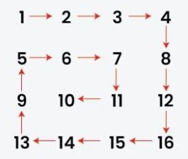
Employ boundary traversal technique.

Example: 
Input: mat[][] = {{1,  2,  3,  4,  5}, 
                  {14, 15, 16, 17, 6},
                  {13, 20, 19, 18, 7},
                  {12, 11, 10, 9,  8}};

The input numbers have been given in spiral form, and should just be read.

Output : 1, 2, 3, 4, 5, 6, 7, 8, 9, 10, 11, 12, 13, 14, 15, 16, 17, 18, 19, 20

Solution

The algorithm is as follows:

- Traverse the top row from j=0 to j=m-2.
- Traverse the rightmost column from i=0 to i=n-2.
- Traverse the bottom row from j=m-1 to j=1.
- Traverse the leftmost column from i=n-1 to i=1.

- Traverse the second row from j=2 to j=m-3.
- Traverse the last-but-one rightmost column from i=1 to i=n-3.
- Traverse the last-but-one bottom row from j=m-2 to j=2.
- Traverse the second leftmost column from i=n-2 to i=2.

- Traverse the third row from j=3 to j=m-4.
- Continue the traversing in the spiral form. - - -
- - - - - -

The program

The program is (read through the code and comments):

    spirallyTraverse <- function(mat) {
        # Determine dimensions automatically
        n <- nrow(mat)
        m <- ncol(mat)
  
        # Let a be the difference between the row being traversed, and i=1.
        # Let b be the difference between the column being traversed, and j=1.
        a <- 1
        b <- 1
        # Let c be the difference between the bottom of the matrix and the traversing column end element index.
        # Let d be the difference between the right end of the matrix and the traversing row end element index.
        c <- n
        d <- m
  
        totalNumOfElements <- n * m
        counter <- 0
        i <- 1; j <- 1
  
        while (counter < totalNumOfElements) {
            # Traverse top current row from left to right
            for (j in b:d) {
              cat(mat[a, j], ", ", sep = "")
              counter <- counter + 1
            }
            j <- d # Update j to its last loop value
    
            # Traverse last current column from top to bottom
            for (i in (a + 1):c) {
                cat(mat[i, j], ", ", sep = "")
                counter <- counter + 1
            }
            i <- c # Update i to its last loop value
    
            # Traverse current bottom row from right to left
            if (a < c) {    # Check to avoid duplicating row in single-row matrix
                for (j in (d - 1):b) { 
                    cat(mat[c, j], ", ", sep = "")
                    counter <- counter + 1
                }
                j <- b
            }
    
            # Traverse current first column from bottom to top
            if (b < d) {    # Check to avoid duplicating column in single-column matrix
                for (i in (c - 1):(a + 1)) {
                    cat(mat[i, j], ", ", sep = "")
                    counter <- counter + 1
                }
                i <- a
            }
    
            a <- a + 1; b <- b + 1; c <- c - 1; d <- d - 1
        }
        
        cat("\n")
    }   

# main area
    mat = matrix(c(1,  2,  3,  4,  5, 
                   14, 15, 16, 17, 6,
                   13, 20, 19, 18, 7,
                   12, 11, 10, 9,  8), nrow = 4, ncol = 5, byrow = TRUE)
          
    spirallyTraverse(mat);

The output is:

1, 2, 3, 4, 5, 6, 7, 8, 9, 10, 11, 12, 13, 14, 15, 16, 17, 18, 19, 20,

The time complexity is actually O(2 n x m), with the first O(n x m) for populating the input matrix with all the elements, and the second O(n x m) for iterating over all the elements in the matrix in the called function. Since the coefficient (multiplicand of 2) is usually omitted, the time complexity is quoted as O(n x m).

The space complexity is O(n x m), for the input matrix, which is the same as the matrix in the called function (same reference).

Thanks for reading.